IPFS

knowledge should be freely accessible to all

Institute for Plasma Focus Studies

Internet Workshop on Numerical Plasma Focus Experiments

Module2; (Follow the instructions in the following notes. You may also wish to refer to the supplementary notes part2supplementary.htm

Summary:

For this module we fit model parameters so that computed current waveform matches measured current waveform.

First we configure the UPFL for PF1000 operating in Deuterium; using trial model parameters. We fire a shot. We do not know how good our results are without a reference point; ie some comparison with experimental results.

A total current waveform of the PF1000 has been published; we have it in digitized form.

To ensure that our computed results are comparable to experimental results, the key step is to fit model parameters, by adjusting the model parameters until the computed total current trace matches the measured total current trace.

To do this, we add a Sheet 2 to our numerical plasma laboratory; place the digitized data of the measured trace in Sheet 2 and plot this trace in a chart. Next we plot the computed current waveform in the same chart. The model parameters are varied; at each variation the focus is fired, and the computed current waveform is compared with the measured waveform. The process is continued until the waveforms are best matched. A good match gives confidence that the computed results (trajectories, speeds, temperature, neutron and radiation yields etc) are comparable with actual experimental results.

After the guided fitting of the PF1000, we have a self exercise to fit the Chilean PF400.

We then tabulate important results of both machines, and do a side-by-side comparison of a big vs a small plasma focus to obtain important insights into scaling laws/rules of the plasma focus family.

Steps: (a) To configure the code for the PF1000 using trial model parameters

(b) To place a published PF1000 current waveform on Sheet 2.

(c) To place the computed current waveform on Sheet 2 in the same figure

(d) To vary the model parameters until the two waveforms have the best match.

(e) Exercise 2: Tabulate results for PF1000 obtained in our numerical experiment.

(f) Exercise 3; participants to fit the PF400 and tabulate the results for PF400 side by side with the results for PF1000, for a comparative study.

The material:

You need File7RADPFV5.15b (called File7) for the following work. Copy and Paste a copy on your Desktop. You also need the files PF1000data.xls, PF400data.xls and compareblank.xls for this session. Use the cursor to drag each file onto your desktop.

(a) Configure the code for PF1000

Double click on File7 (Excel logo File7RADPFV5.15 on your Desktop).

Security pop-up screen appears.

Click on enable macros

The worksheet opens.

[Type in cell B3: PF1000; for identification purposes.]

[The PF1000, at 40kV, 1.2 MJ full capacity, is one of the biggest plasma focus in the world. Its 288 capacitors have a weight exceeding 30 tonnes occupying a huge hall. It is the flagship machine of the ICDMP, International Centre for Dense Magnetised Plasmas.]

We use the following bank, tube and operating parameters:

Bank: L_o=33.5 nH, C_o=1332 mF, r_o=6.3mOhm

Tube: b=16 cm, a=11.55 cm, zo=60 cm

Operation: V_o=27kV, P_o=3.5 Torr, MW=4, A=1, At-Mol=2

For this exercise we do not know the model parameters. We will use the trial model parameters recommended in the code (See cells P9-V9)

Model: massf=0.073, currf=0.7, massfr=0.16, currfr=0.7; our first try.

Configuring: Key in the following:

A5 B5 C5 D5 E5 F5

33.5 1332 16 11.55 60 6.3

Then A9 B9 C9 D9 E9

27 3.5 4 1 2

Then A7 B7 C7 D7

0.063 0.7 0.16 0.7 for first try

Or follow the guide in A4-F4, to key in A5-F5 for the relevant parameters.

Fire a shot: Place the cursor in any blank non-active space, e.g. G8. (point the cursor at G8 and click the mouse). Press ‘Ctrl’ and ‘A’. (equivalent to firing a shot)

The program runs and results are displayed in columns and also in figures.

Is our simulation any good? Not if there is no reference point!!

To assess how good our simulation is, we need to compare our computed current trace with the measured current trace, which has been published.

Note that at this point: File7 contains computed data for PF1000 with the trial model parameters of: massf=0.073, currf=0.7, massfr=0.16, currfr=0.7

(b) To place a published PF1000 current waveform on Sheet 2

(i) The PF1000 current waveform is in the file PF1000data.xls. You now want to place this data into File7 as Sheet2. With File7 open, click on ‘File’ tab; drop down appears, click on ‘Open’. Look in: Desktop; select PF1000data.xls; double click to open this file. Click on ‘Edit’ tab; select ‘Move or Copy Sheet’. A window pops out; ‘Move selected sheets To book’; select ‘File7RADPF13.9b.xls. ‘Before Sheet:’ select ‘(move to end)’. Click ‘OK’. You have copied PF1000data.xls into File7 as Sheet1(2); you might like to rename Sheet1(2) as Sheet2.

(ii) Chart the measured current waveform: The measured current waveform is already charted in Sheet2. You may adjust the size and position of the chart for your preferred viewing.

(c) To place computed current waveform on Sheet 2 in the same chart

To place the computed current waveform on the same chart: Position the cursor on the chart containing the measured current waveform. Now right click. Pop-up appears. Select ‘Computed Current in kA’ in the name box.

In the next steps we will place the computed current data from Sheet 1 into this same chart in Sheet 2, by the following procedures. Place the cursor in the box against ‘X values’ by clicking. Then type in the following string: “=sheet1!$a$20:$a$6000” [without the quotation marks]. Next click in the box against ‘Y Values’ and type in the following: “=sheet1!$b$20:$b$6000” [without the quotation marks]. Click button ‘OK’.

The pink trace (see figure below) is the computed current trace transferred from Sheet 1 (where the time data in us is in column A, from A20-Aseveralthousand; and corresponding computed current data in kA is in column B, from B20 to B severalthousand). We are selecting the first 5980 points (if that many points have been calculated) of the computed data; which should be adequate and suitable.

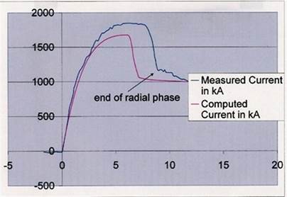
Comparison of traces: Note that there is very poor matching of the traces; using the first try model parameters.

(d) Vary model parameters to obtain matching of computed vs measured current traces. (bank, tube & operating parameters all given correctly)

(i) First fit the axial phase:

[suggestion: read part2supplementary.doc pg 2 bottom para ‘First step is fitting axial phase’.]

From the comparison chart on sheet 2,

We note: that the computed current dip comes much too early;

that the computed current rise slope is only very slightly low;

that the computed current maximum is too low.

All these 3 observations are consistent with a possibility that the axial speed is too fast; which would cause the radial phase to start too early. Too high an axial speed would also cause too much loading on the electrical circuit (similar to the well known motor effect) as the quantity [0.5*dL/dt=0.5x L’*dz/dt] is a dynamic resistance loading the circuit

during the axial phase; here the inductance per unit length L’=(m/2p)*ln(b/a) This too high speed would also lower the peak current.

To reduce the axial speed, we could increase the axial mass factor. We note that the axial phase ends too early by some 20%; indicating the axial speed is too fast by 20%.

In the plasma focus (as in pinches, shocks tubes and other electromagnetically driven plasma devices) speed~density^0.5. So the correction we need is to increase the axial mass factor by 40%. So try an axial mass factor of 0.073x1.4~ 0.1.

We toggle to Sheet 1 by clicking on ‘Sheet 1’ (just below the worksheet).

Click on cell A7, and type in 0.1.

Fire the focus by pressing Ctrl+A.

Program runs until complete, and results are presented.

Note TRadialStart (H16) has increased some 0.7 us.

Toggle to Sheet 2 (ie click on Sheet 2 just below work sheet).

Note that the computed current dip is now closer to the measured in time (still short by some 10%; reason being that increasing axial mass factor reduces the speed which in turn causes a reduced loading. This increases the current which tends to increase the axial speed so that our mass compensation of 40% becomes insufficient). The value of the computed peak is also closer to the measured. So we are moving in the right direction!

But still need to move more in the same direction. Next try axial mass factor of 0.12. Toggle to Sheet 1, type 0.12 in A7. Fire. Back to Sheet 2. Note improvement in all 3 features.

In similar fashion, gradually increase the axial mass factor. When you reach 0.14 you will notice that the computed current rise slope, the topping profile, the peak current and the top profile are all in good agreement with the measured. The computed trace agrees with the measured up to the start of the dip. Note that the axial model parameters at this stage of agreement are: 0.14 and 0.7. You may wish to try to improve further by making small adjustments to these parameters. Or else go on to fit the radial model parameters.

(ii) Next, fit Radial phase:

Note that the computed current dip is not steep enough, and dips to too low a value. This suggests the computed radial phase has too high a speed. Try increasing the radial mass factor (cell C7), say to 0.2. Observe the improvement (dip slope becomes less steep) as the computed current dip moves towards the measured.

Continue making increments to massfr (cell C7). When you have reached the massfr value of 0.4; it is becoming obvious that further increase will not improve the matching; the computed dip slope has already gone from too steep to too shallow, whilst the depth

of the dip is still excessive.

How to raise the bottom of the dip? Here we suppose the following scenario:

Imagine if very little of the current flows through the pinch, then most of the total current will flow unaffected by the pinch. And even if the pinch were a very severe one, the total current (which is what we are considering here) would show hardly a dip. So reducing the radial current fraction, ie currfr (or f_cr) should reduce the size of the dip.

Let us try 0.68 in cell D7. Notice a reduction in the dip. By the time we go in this direction until currfr is 0.65, it becomes obvious that the dip slope is getting too shallow; and the computed dip comes too late.

One possibility is to decrease massfr (which we note from earlier will steepen the dip slope); which however will cause the dip to go lower; and it is already too low.. Another possibility is to decrease the axial phase massf, as that will also move the computed trace in the correct direction.

Try a slight decrease in massf, say 0.13.

Note that this change aligned the dip better but the top portion of the waveform is now slightly low, because of the increased loading on the electrical circuit by the increase in

axial speed. This suggests a slight decrease to circuit residual resistance r_o ( or changes to L_o or C_o; fitting those could be tricky, and we try to avoid unless there are strong reasons to suspect these values). Easier to try lowering r_o first. Try changing r_o to 6.1 mW.

The fit is quite good now except the current dip could be steepened slightly and brought slightly earlier in time. Decrease massfr, say to 0.35. The fit has improved, and is now quite good, except that the dip still goes too low. At this stage we check where we are at.

Toggle to sheet 1. Note from sheet 1 that the radial phase ends at 9.12 ms. Back to sheet 2.

Observe (using cursor) that the point 9.12 is not at the point where the computed (pink curve) dip reaches its inflection point; but some 0.02 ms before that point. (see fig below)

So we note that the computed curve agrees with the measured curve up to the end of the radial phase with a difference of less than 0.02MA out of a dip of 0.66MA (or 3%).

The fitting has already achieved good agreement in all the features (slopes & magnitudes) of the computed and measured total current traces up to the end of the radial phase.

Do not be influenced by agreement, or disagreement of the traces beyond this end point.

The best fit?

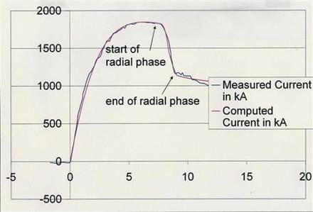
So we have confidence that the gross features of the PF1000 including axial and radial trajectories, axial and radial speeds, gross dimensions, densities and plasma temperatures, and neutron yields up to end of radial phase may be compared well with measured values.

Moreover the code has been tested for neutron and SXR yields against a whole range of machines and once the computed total current curve is fitted to the measured total current curve, we have confidence that the neutron and SXR yields are also comparable with what would be actually measured.

[Having said that, those of you who have some experience with the plasma focus would note that at the end of the radial phase, some very interesting effects occur leading to a highly turbulent situation with occurrence, for example, of high density hot spots. These effects are not as yet modeled in the code. Despite this drawback, the postulated beam-target neutron yield mechanism seems able to give estimates of neutron yield which broadly agree with the whole range of machines. For example, the neutron yield computed in this shot of 8.6x10^10 is in agreement with the reported PF1000 experiments.]

(e) Exercise 2:

Fill in the following:

Q1: My best fitted model parameters for PF1000, 27kV 3.5 Torr Deuterium are:

f_m= f_c= f_mr= f_cr=

Q2: Insert an image of the discharge current comparison chart in Sheet 2 here.

Q3

Fill up the following table. Use the file compareblank.xls for this purpose.
Parameter	PF1000
	( at 27kV 3.5 Torr D2)
Stored Energy Eo in kJ
Pressure in Torr, Po
Anode radius a in cm
c=b/a
anode length zo in cm
final pinch radius rmin in cm
pinch length zmax in cm
pinch duration in ns
rmin/a
zmax/a
Ipeak in kA
Ipeak/a in kA/cm
S=(Ipeak/a)/(Po^1/2)( kA/cm)/Torr^1/2
Ipinch in kA
Ipinch/Ipeak
Peak induced voltage in kV
peak axial speed in cm/us
peak radial shock speed cm/us
peak radial piston speed cm/us
peak temperature in 10^6K
neutron yield in 10^6

[After filling, save this Excel sheet You will use the same Excel sheet to fill in the results for PF400 which is the subject of the next exercise.]

(f) Exercise 3: Participant to fit computed current to measured current waveform of PF400 (bank, tube and operating parameters all correctly given)

In Modulek 1, we worked with the Singaporean NX2; a 3kJ neon plasma focus designed for SXR lithography. This week we worked with the Polish PF1000, one of the largest plasma focus (MJ) in the world. You are now given data for the PF400, a small sub-kJ plasma focus operated in Chile at the Atomic Energy Commission, for the specific purpose of investigating small focus devices. [note: The 1000 in PF1000 refers to kJ. The 400 in PF400 refers to J; so the energy ratio of the PF1000 to the PF400 is: 1,200,000/400~3000]

Given: the current waveform data of the PF400, digitized from a published waveform. The data is in the file PF400data.xls.

Your job: is to fit model parameters until the computed current waveform matches the measured waveform. Some guidance is given below.

Suggested steps to fit PF400:

Copy a clean copy of File7RADPF05.14.xls (called File7) from your Reference folder to your Desktop. Open File 7.

Copy PF400data.xls into Sheet2 of File7. The measured waveform is already pre-charted

Transfer computed current data from Sheet 1 onto Sheet 2; using strings: “=sheet1!$a$20:$a$6000” [without the quotation marks] &: “=sheet1!$b$20:$b$6000” [without the quotation marks]. No trace of computed current appears yet, since we have not yet ‘fired’ PF400.

Write down the bank, tube and operating parameters (from the table in the lower part of the page, NOT from the top line, which contains some nominal values). Toggle to Sheet 1.

Configure the Universal Plasma Focus:

Key in the following bank and tube parameters and the operating parameters.

Lo(nH)	Co(uF)	b(cm)	a(cm)	zo(cm)	ro(mohm)
40	0.95	1.55	0.6	1.7	10
MASSF	CURRF	MASSFR	CURRFR	Model Parameters
Vo(kV)	Po(torr)	MW	At No.	At1;Mol2	Operation Parameters
28	6.6	4	1	2

Key in the first try model parameters; [scroll a little to the right and use the suggested parameters for the UNU ICTP PFF, cells T9-V9].

Fire PF400; and see the comparative results by toggling to Sheet 2.

Fitting the computed current waveform to the measured waveform:

Suggested first steps: Fit the axial region by small adjustments to f_m and f_c, where necessary. In fitting the axial phase, the more important region to work on is the later part of the rising slope and the topping profile towards the end of the axial phase. So each time you should note the position of the end of the axial phase from Sheet 1 and locate that position on the Chart in Sheet 2, using the cursor.

Final steps: When you have done the best for the axial phase up to the end of the axial phase, then proceed to fit the radial phase. Tip: The dip for the PF400 is not very dramatic. Enlarge the trace so the rollover and the dip can be more clearly compared.

(f) Exercise 3:

Fill in the following, copy and paste and e-mail to me by 26 April 2008.

Q1: My best fitted model parameters for PF1000, 27kV 3.5 Torr Deuterium are:

f_m= f_c= f_mr= f_cr=

Q2: Insert an image of the discharge current comparison chart in Sheet 2 here.

Q3: Complete the Excel Sheet which you started in the last Exercise; to compare a BIG (~500kJ) plasma focus with a small one (~400J). As you fill up, note particularly each group of ratios (each group is denoted by a different colour). Note particularly the order of magnitude of the ratios. [use the Excel sheet, rather than this table].

The ratios below were calculated from the actual PF1000 and PF400 results; and left here as a check for you. Calculate your own ratios from your own results. At the end of the exercise save this Excel Sheet as PFcomparison.xls. It will be used again next week.

Make up the following table comparing a BIG plasma focus with a small one.
Parameter			PF1000	Ratio		PF400
			( at 27kV 3.5 Torr D2)	PF1000/PF400		(at 28kV 6.6 Torr D2)
Stored Energy Eo in kJ			486	1313		0.37
Pressure in Torr, Po			3.5	0.53		6.6
Anode radius a in cm			11.55	19.3		0.6
c=b/a			1.39	0.54		2.6
anode length zo in cm			60	35.2		1.7
final pinch radius rmin in cm				26.7
pinch length zmax in cm				22.2
pinch duration in ns				53
rmin/a				1.4
zmax/a				1.16
Ipeak in kA				14.6
Ipeak/a in kA/cm				0.76
S=(Ipeak/a)/(Po^1/2)( kA/cm)/Torr^1/2				1.05
Ipinch in kA				9.64
Ipinch/Ipeak				0.65
Peak induced voltage in kV				2.4
peak axial speed in cm/us				1.24
peak radial shock speed cm/us				0.48
peak radial piston speed cm/us				0.48
peak temperature in 10^6K				0.19*
neutron yield Yn in 10^6				81920
Measured Yn in 10^6: range			(2 - 7)E+03			0.9-1.2
Measured Yn in 10^6 :highest			2.0E+04
	Note: ratios in orange: values are of the order of 1; ratios in blue: values are of the order of (ratio of anode radii)
	or (ratio of Ipeak); ratio of temperature (orange*) is a special case, because of the difference in values of c.
	[These points are worth thinking about; with reference to the file on the Theory of the Lee model,
	available from http://www.plasmafocus.net/
	Look especially at the sections on the scaling parameters of the axial and radial phases]
This table summarises the results of our numerical experiments for Week 2 of the course.
It could be the start of a compilation covering all focus machines for which measured current traces are available.
We could then use the tabulation for several uses including the following:
Think of scaling rules, laws:
1. How does rmin, zmax, and pinch duration, scale primarily with anode radius 'a'? Should there be a relationship?
2. How does the (pinch volume*pinch duration) scale with 'a'?					Should there be a relationship?
3. What is the significance of the Speed Factor S?
[hint: speed factor S is a measure of the axial speed; it is also a measure of the energy per unit mass during the axial phase;
also a measure of the energy per unit mass of the radial phase, however the radial phase speeds*** relative to the axial phase
speed are modified by a factor [(c^2-1)/lnc]^0.5; so for 2 devices if the axial speeds are the same and c is the same,
one would expect the radial speeds to be essentially the same. In that situation the temperatures would also be essentially
the same. Following this line of argument, can you see why there should be a big difference between the temperatures
of PF1000 and PF400? Which one's temperature should be higher?]
4. How should the neutron yield scale? With storage energy E, with Ipeak, with Ipinch?
		Papers\PP2 with Erratum JoFE NeutronScalingLawsFromNumericalExperiments.pdf

***The ratio radial speed/axial speed is:

is http://www.plasmafocus.net/

download the Theory of the model

Conclusion:

In these two sessions we have learned how to fit a computed current trace with a measured current waveform, given all bank, tube and operational parameters. For the PF1000 we obtained a good fit of all features from the start of the axial phase up to the end of the radial phases; giving confidence that all the computed results including trajectories and speeds, densities, temperatures and neutron and radiation yields are a fair simulation of the actual PF1000 experiment.

We also fitted the Universal Plasma Focus Laboratory to the PF400.

We tabulated important results of the two machines side by side.

We noted important physics:

that although the machines differ greatly in storage energy and hence in physical sizes, the speed factor S is practically the same. This has given rise to the now well-known observation that all plasma focus, big and small, all operate with essentially the same energy per unit mass when optimized for neutron yield, see e.g.: http://en.wikipedia.org/wiki/Dense_plasma_focus

The axial speed is also almost the same; in which case the radial speeds would have been almost the same, except they (the radial speeds) are influenced by a geometrical factor [(c^2-1)/lnc]^0.5. For these 2 machines the factors differ by 1.5; hence explaining the higher radial speeds in PF400; and also the higher temperatures in the smaller PF400.

The pinch dimensions scale with ‘a’ the anode radius. The pinch duration also scales with ‘a’, modified by the higher T of the PF400, which causes a higher small disturbance speed hence a smaller small disturbance transit time. In this model this transit time is used to limit the pinch duration.

Finally we may note that just by numerical experiments we are able to obtain extensive properties of two interesting plasma focus machines apparently so different from each other, one huge machine** filling a huge hall, the other a desk top device. Tabulation of the results reveal an all important characteristic of the plasma focus family. They have essentially the same energy per unit mass (S ). A final question arising from this constant energy/unit mass: Is this at once a strength as well as a weakness of the plasma focus?

End of Part 2